Yearly Archives: 2014

electronics

3D Printing and Custom Enclosures

I finally got around to finishing my Jeep computer project. I had gotten the Arduino and display working, and I had wired everything together. However, as of my previous post about the project, neither the display nor the Arduino were in enclosures, and the cabin of the Jeep was festooned with wires.

The first step in cleaning up the mess was to purchase an inexpensive, generic, plastic, rectangular enclosure from Radio Shack. I drilled some holes to mount the connections for the Arduino/GPS unit. I put it together and tucked it behind the dash, nice and neat. So most of the wires were gone. The only remaining messy part was the display. I still had the bare display nestled e’er so gently in a knit cap that I’d leave on top of the dash as a pillow for my electronics. I wanted an enclosure that would fit snugly around the display, and that I could mount on the dashboard.

At some point along the way, I learned that the Washington DC public library system has a 3D printing service. For a minimal cost, they would make a print of an object. Fantastic! I just needed to figure out how to create a model. I learned that I was going to need to use a CAD program to create an .stl (STereoLithography) file, which seems to be one of the primary file formats in the 3D printing world.

Of course, I didn’t want to spend thousands of dollars on a CAD program that would take years to learn. Fortunately, there are free, easy-to-learn options, such as SketchUp or TinkerCAD. SketchUp is a native program that runs on Macs and Windows computers. While I have a couple of Macs, and I run various versions of Windows in virtual machines for testing purposes, at home, my primary computer is Linux. TinkerCAD is a very simple, web-based CAD program that works well in any modern browser.

After a basic exploration of TinkerCAD, I was ready to go about designing the custom enclosure for my display. The display is a 2.8″ TFT LCD Touchscreen Breakout from Adafruit. I spent some time searching for specs that list the dimensions, but no such specs were to be found. So I pulled a tape measure out of my knitting kit, and built the CAD model as I measured the dimensions.

TinkerCAD and the Display

My first attempt included a back plane. Having no experience with 3D printing, I didn’t realize that in order to support the back plane during the printing process, the printer would have to lay down a grillwork of plastic that I would have to remove after the fact.

3D Grillwork

I attempted to remove the grillwork, but the plastic is surprisingly sturdy. (In fact, I was originally worried that the 2mm walls of my model would be flimsy, but it ended up being rock solid… Err, in a plastic sort of way.) So I removed the back in the CAD file, and resubmitted. I got back an enclosure that fits the display perfectly.

Enclosure

Enclosure

Enclosure

Enclosure

I considered adding grooves to the enclosure so I could print a separate back plane that could be attached and detached. In the end, I went with simplicity, and I just used a bit of Gorilla Tape for the back. I’ve mounted it on the dashboard (again, with Gorilla Tape until I settle on a more permanent solution), and it satisfies all of my greatest hopes and desires (with respect to a 3D printed enclosure anyway).

Enclosure

Enclosure


electronics

Jeep Seat Heaters

Once you own a car with seat heaters, it’s hard to go back. The old VW had heated seats; the new Jeep did not. Clearly, this state of affairs could not stand.

I found that I could get some nice, neoprene seat covers with built-in seat heaters made by Wet Okole. The Wet Okoles came with heating elements in both the butt-area and the back-area, whereas some aftermarket heaters only heat the butt. I used Quadratec’s “designer” for Wet Okoles. When the seat covers arrived, I installed them, and there was much rejoicing.

Wet Okole Seat Covers

Each seat had a cigarette lighter plug for power, and a push-button switch that allowed setting the heater element to Off, Low, Medium, or High.

Original Switch

Here we get to the problem: While convenient for a quick connection, I didn’t want wires dangling from the seats to the cigarette lighter. Further, I only had one cigarette lighter. Even splitting the circuit for the cigarette lighter wasn’t a great solution, as each seat could potentially draw a little more than 10 amps, and the lighter was on a 20 amp fuse. Splitting the circuit would mean that I’d risk blowing the fuse each time both seats were on full. The Jeep conveniently has a spare 20 amp circuit on the fuse block behind the dash, but it’s an unswitched circuit. If I used that, it’d only be a matter of time before I’d leave the car with a seat heater on, and I’d come back to a dead battery.

After using the seat heaters for a while, I decided that they were keepers, so it was worth investing in a more permanent solution to the power problem — and a solution that would allow both seats to be heated at the same time. I needed to add at least two new 15 or 20 amp, switched circuits to the car, and I wanted controls that were integrated into the dashboard somehow.

For the controls, I started looking around for switches that could put into some existing blanks on the dash. However, after bashing in a heater vent (by transporting some furniture in the passenger seat), I stumbled upon the perfect solution in a Daystar replacement vent with an integrated switch panel.

Vent Switches

The drawback of the rocker switches is that I would no longer have Low or Medium settings. The seat heaters would either be off, or fully on. But really, who need a “lightly warmed” bum in winter? If it’s cold enough to turn ’em on, turn ’em on ALL THE WAY, I say!

For the circuits, I found that Painless Performance makes three- and seven-circuit add-on fuse blocks. I decided to go with the seven-circuit block to give me room for expansion in future, yet-to-be-conceived projects (such as my Arduino-based trip computer). That gave me four new switched circuits, and three new constant circuits, all at 20 amps.

The parts arrived, and so I got to connecting all the pieces. The trickiest decision was where to mount the new fuse block. I had initially intended to mount it behind the glove compartment, next to the existing internal fuse block, but there wasn’t enough room. Perhaps I could have found another spot behind the dash, but I didn’t want to put it somewhere that would require ripping open the dash to access it (in case I should need to replace a fuse). There was an empty spot in the engine compartment (for a second battery, I suppose, to power a winch that I’m unlikely to add) that seemed like a good candidate. Being in the engine compartment, I wanted to add a bit of protection to the block, as it wasn’t marketed as a weatherproof component. So rather than mounting it directly, I mounted it to the inside of a small tupperware bin. I drilled a few ventilation holes in the bin, and a larger hole to run the wires, then mounted the bin in the engine compartment.

Placement of fuse block

The new fuse block is in a ventilated tupperware bin, mounted near the back-driver-side of the engine compartment.

The fuse block had three sets of wires:

  1. Two wires to connect to the positive and negative poles of the battery to power the circuits.
  2. A single wire that needed to be connected to an existing switched circuit. This wire poweres an internal relay that controlled the switching of the four switched circuits in the fuse block.
  3. Seven hot wires for the seven new circuits.

Since the fuse block was already in the engine compartment, running the first set of wires to the battery was fairly trivial. The rest of the wires, though, had to make it into the cabin, which meant getting them through the firewall. I spent more than a few minutes looking for an accessible, existing run through the firewall, and was met with no success. I refered to Dr. Google, and learned that a hard, rubber plug near the gas pedal is the preferred channel — just make a hole straight through it. I made the hole, and pulled the wires through.

Wires run through the firewall

To get the wires through the firewall, I had to make a hole in a rubber plug that seemed to exist for exactly that purpose.

For the relay wire, I tapped into the hot line for the cigarette lighter — I just cut away a centimeter of insulation, joined the relay wire, and wrapped it up neat and tidy with electrical tape. The remainder of the work consisted of running wires up and down behind the dash: hot circuit wires to switches, switches to positive wires for the seats, switches to ground, seats to ground.

As of this blog post, the seats have been keeping my bum warm for more than two winters. A boy could hardly ask for more.

Switches

programming

UltraSignup Visualizer


Instructions

  • In the text box at the top of the graph, enter the full name of a runner whose results can be found on UltraSignup, then hit enter.
  • The points on the graph represent individual race results for the given runner. Move your mouse over a point to see details of that race.
  • The line represents the evolution of the runner’s UltraSignup rank.
  • Timed events (eg, 12-hour races, 24-hour races) appear as empty circles. It seems that as of mid-October, 2014, timed events are included in the ranking. However, it is not clear to me if that change is retroactive, and in some circumstances, I cannot get my calculation of the ranking to line up with their calculation of the ranking. So if you have a large number of timed events in your history, the line I’ve calculated might be e’er so slightly off. The ranking reported below the graph is the official number, provided by UltraSignup.

Background

[Update: The friendly folks at UltraSignup came across this, and they liked it. I worked with them to get it integrated into the official runner results page. So now you can click the “History” link just below a runner’s overall score on UltraSignup and see the plot on the results page. Though if you like the spanky transitions between runners, you still need to come here.]

In the world of ultrarunning, it seems that the ranking calculated by UltraSignup has become the de facto standard for ranking runners. I think that part of the reason for its acceptance is its simplicity. A runner’s rank in a single race is just the ratio of the winner’s finish time to the runner’s finish time. So if you win a race, you get a 100%; if you take twice as long as the winner, you get a 50%. The overall ranking is a single number that represents an average of all of a given runner’s race rankings. If you were to look up my results on UltraSignup, you would see that as of this moment of this blog post, my 10+ years of racing ultras has been boiled down to a ranking of 88.43% over 48 races.

Of course, with simplicity comes inflexibility. What that number doesn’t capture is change over time. By summing up my results as a single number, it’s hard to see how my last few years of Lyme-impaired running have affected my rank, or how my (hoped-for) return to form will affect it. I was curious to see how runners progress over time, and how it affects the UltraSignup rank. In looking at the details of how UltraSignup delivers their rank pages, I noticed that the results come as JSON strings. Therefore, I realized, I wouldn’t even have to do any parsing of irregular data. I could just pull the JSON, and use my handy D3 skillz to put the results in a scatter plot.

I won’t go into great depth about implementation details. If you happen to be interested, you can go to the source. A passing familiarity with D3 would be helpful, but familiarity with only vanilla Javascript should allow you to get the gist.

Oh, and be aware that since this pulls data from UltraSignup, it’s entirely possible that it will stop working someday, either because they change the way they deliver data, or because they don’t like third parties creating mashups with their data. Also, this doesn’t work on Internet Explorer 8, or earlier. Sorry ’bout that!

programming

Revoice

Some years ago, I was in need of a new and unique way to taunt a friend. He had made a habit of being especially obnoxious in an certain online forum. But it’s not his obnoxiousness that really bothered me. In fact, many friends and acquaintances would consider me to be chief among purveyors of obnoxiousness.  No… It’s not the obnoxiousness that bothered me. It was the repetition within the obnoxiousness that brought me to action. Every day, it was the same rants, the same complaints, the same stock phrases.

I had, for some time, tried to taunt him by twisting his words, offering clever (according to me) puns, countering him with facts and offering the straight-up observation that he was saying the same thing, day after day. It was like throwing spitballs at a steamroller. Clearly, I needed to step up my game.

My first thought was to compile his most-used stock phrases, create bingo cards with them and distribute those cards to other participants of the forum. That way, even if we had to put up with this repetitive obnoxiousness, at least we could derive some fun from it—and maybe someone could win a prize!

As much fun as that might have been, I decided that I wanted something unique, and bingo had been done. (It hadn’t been done in this particular case. But I wasn’t the first one to think of creating a bingo game based on the phrases someone frequently says.) So I came up with the idea of writing a program that would generate new posts for the forum. The posts would be in the style of the individual of my choosing—using the same vocabulary and phrasing—but would essentially be nonsense. This idea had that dual benefits of being an effective method of taunting as well as being an interesting project.

I had forgotten about this little project for many years. Recently, though, I came across an old, broken laptop. I knew that this laptop had some old projects on it (including a simple 3D drawing program I wrote in college, and some signal processing and computer learning code I had written for a long-extinct dot-com that rode that early-2000s bubble with the best of ’em). I decided to pull the data off the hard drive (a process that ended up being quite a project in itself). I thought my taunting program might be on that disk. But it was nowhere to be found. After some more thought about where and when I wrote the program, I realized that I had written it on a computer from a later era that had since experienced a catastrophic disk failure.

Rather than being disappointed that I had lost that little gem, I decided to recreate it. I recalled that I had written it as a short PERL script that only took a couple hours to code. Although I haven’t touched PERL in six or seven years (other than to make trivial tweaks to existing code), I remembered the premise on which I based the original program, and PERL is certainly the best readily-available tool for this job.

To understand how the program works, you need to understand that everyone has characteristic patterns in their writing or speech—a sort of linguistic fingerprint, or voiceprint. You can do all sorts of analysis on an individual’s language to determine various aspects of that voiceprint. The trick is to find some set of aspects that are not only descriptive, but that could be used generatively.

One component of that voiceprint is vocabulary—the set of words that someone knows and uses. So I could take some sample text, extract the vocabulary used in that text, and use those words in random order. Unfortunately, that would end up as a jumbled mess. The first problem is that most of us share the majority of our vocabulary. There are a few hundred words that make up that majority of what we say. It’s only at the periphery of our vocabulary—words that hold some very specific meaning and that are used infrequently, like “periphery”—where we start to notice differences.

To accomplish my goal, I was going to need a system that would not only use the same words that are in a sample text, but would also use them in a similar, but novel, way. I could take the idea from above—to use the vocabulary—and add the notion of frequency. That is, I wouldn’t just randomly pick words from a vocabulary list. Instead, I would note the frequency of each word used, and pick words with the same probability. For example, if the word “the” makes up 3% of the sample text, then it would have a 3% likelihood of being picked at any particular step in the generated text.

But we still have the problem that the resulting text wouldn’t have any coherence beyond the word level. It would just be a jumble of words strung together. To add coherence, we need context. Context means that we need to look at the way that words are strung together. We can do that by looking at tuples—ordered sets—of words. For the sake of settling on a reasonable number, let’s pick 3. Let’s look at 3-tuples. This paragraph starts with the 3-tuple {But,we,still}. The next 3-tuple is {we,still,have}. Then {still,have,the}, then {have,the,problem}, and on and on.

Looking at tuples, we get a small amount of context.  My question when I started this project was whether that context was enough to build a generative system that could speak in the voice of some training text. Since the tuples are sequences that appear with some known frequency, and since one tuple could be chained to the next by using those known frequencies, I had high hopes.

To understand how this would work, we could train it on a piece of my own writing: my Hellgate 100k race report from 2007. Say I was in the middle of generating new text based on that post, using 3-tuples. Now, say that last two words in my generated text are “going to”. (Forget about how I reached that point, just assume that I’m there.) I need to pick the next word. Based on earlier analysis, I know that the following table shows all of the 3-tuples taken from that post, which start with {going,to}. The number next to each 3-tuple is the number of times the 3-tuple appears in the post.

{going,to,run} (1)
{going,to,win} (1)
{going,to,be} (1)

To be consistent with the sample text, the next word needs to be “run”, “win” or “be”. Based on the frequencies, there is an equal chance of choosing any of the options. Now say that of those options, with those frequencies, we happen to choose “be” as the next word. Our generated text is “going to be”. So we start over, looking for the tuples that start with {to,be}.

{to,be,able} (2)
{to,be,here} (1)
{to,be,very} (1)
{to,be,a} (1)
{to,be,of} (1)
{to,be,running} (1)
{to,be,jogging} (1)
{to,be,at} (1)
{to,be,gathered} (1)

Let’s pick “running”, making our generated text “going to be running”. And on to the next step.

{be,running,for} (1)
{be,running,.} (1)
{be,running,at} (1)

We pick “at”, resulting in “going to be running at”. We are starting to get some text that appears to be somewhat familiar (if you’ve read the sample text) and is syntactically correct, but might be entirely new. (Notice that one of the options in the above example is punctuation. By tokenizing some punctuation—such as periods and commas—the resulting text seems to be more natural.)

The next problem is figuring out how much training text is required to allow the system to generate new text. With a very small amount of training text, the result would not be very interesting. That is because of the relationship between the number of unique 2-tuples and unique 3-tuples. When choosing a new word, we need to look at the final 2-tuple in the generated text. If each 2-tuple is the beginning of only a single candidate 3-tuple—if there is a 1:1 ration between 2- and 3-tuples—then after the first two words are chosen, each additional step will simply extend the generated text with an unaltered section of the source text.

In a very short sample text, the 2- to 3-tuple ratio is likely to be very close to 1:1. As the sample text gets longer, that ratio tends to get smaller.  However, it is not only the length of the text that affects the 2- to 3-tuple ratio; it is also the complexity of the text. Repetition within a text will manifest itself more greatly in smaller portions of text than in larger portions. (Even though they are very close to one another in size, 2-tuples are smaller than 3-tuples, so they will be affected more greatly by repetition.) So a large degree of repetition will result in low 2- to 3-tuple ratio relative to the total length of the text.

It is that second point that drew me to this project. The purpose of this project was to illustrate and emphasize the amount of repetition in an individual’s writing. Therefore, with a relatively small amount of sample text—I collected probably less than 2,000 words of text—the program was able to generate new text in the voice of the original author. Unfortunately, I no longer have that sample text (and the individual in question has stopped posting in that forum).

The race report that I used as an example above has, by my count, 3,687 2-tuples and 4,962 3-tuples, for a ratio of .74. It turns out that that is sufficient to start generating new text. For example, after training on that text, I can generate samples like,

The sixth aid station how far ahead he was ahead of me. Moments later, on a downhill, and I beat the aid station asked how much time I reach Bearwallow Gap. Then I’d restock again, there is a little ball on the leaders. I can do it because I had some soup, hot chocolate, scrambled eggs. I wanted to win, so there was a race. But there were a lot of strong runners on the floor and stomped on until it’s in a little.

Or,

Which brings us to 2007. I felt like there was someone behind me, that’s just post hoc rationalization. Maybe not entirely, but after that, the runner only has the former.

Now we can try to generate something new based on some other text. Hamlet, for example. I took all of the lines that Hamlet speaks in the autonymous play. By my count, in the 11,714 words, there are 10,079 2-tuples and 13,555 3-tuples, resulting in a ratio of .74. Here are some new-and-improved lines for Hamlet:

Let me not burst in ignorance; but, sir, to set on some quantity of choice, To flaming youth let virtue be as wax, And break your own inclining? Is it a free visitation? Come on–you hear this fellow no feeling of his lands will hardly lie in this box; and there is nothing either good or bad, but in the verity of extolment, I pray. The spirit that I have of late–but wherefore I know not of? Thus conscience does make cowards of us all; And now, how cheerfully my mother looks, and on this moor? Ha! have you eyes? Could you on this, The oppressor’s wrong, to hold, as pure as snow, thou shalt not escape calumny.  Get thee to a bawd than the observance. This heavy-headed revel east and west Makes us traduced and tax’d of other nations: They clepe us drunkards, and makes passionate action. The spirit that I know, to this world goes, even in that sleep of death what dreams may come When we have seen, And in this garb, lest I should have fatted all the circumstance?

To be entirely honest, I chose Hamlet because it is a well known work in the public domain. I didn’t really think it through. That certainly looks Shakespearean to me. However, this line of inquiry has made me realize that I can’t necessarily distinguish between actual Shakespearean writing and nonsense that just sounds like Shakespeare.

So I needed something else. I found the 2010 presidential State of the Union address. By my count, in 7,328 words, there are 5,894 2-tuples and 7,649 3-tuples, for a ratio of .77—slightly higher than Hamlet. What do we get from that?

The spirit that has always been our ideals, our values that allowed us to wait for decades, and jeopardize our recovery — all of their income on student loans, and are generous in spirit. These aren’t Republican values or labor values. They’re putting more emphasis on math and science; and turns around failing schools that steal the future was anything but certain. These were the times that tested the courage of our citizens, not our ambitions. So we face big and difficult challenges. And according to the world’s cheapest solar cells or treatment that kills cancer cells but leaves healthy ones untouched.  And when we are responsibly leaving Iraq to its people. Let’s leave behind the fear and division, and I know that some in my own party will argue that we can’t afford it. You hated it. You can see how their money is being spent.

There are some interesting phrases in there. However, it would be interesting to see what happens when processing text with a lower ratio.  I combined the 2001 and 2002 State of the Union addresses to gather a total of 8,221 words. But the ratio of that sample text was the same as the ratio of the 2010 address: .77. So I combined all eight of George W. Bush’s State of the Union addresses. The word count rose to 40,377, and the ratio fell to .64 (24,697:38,632).

Our shared responsibilities extend beyond matters of life and science, and that is precisely what America is the Mayor of Philadelphia. He pursued chemical, and defeatism that refuses to acknowledge that we face a tax increase they do not expect and will not be finished on our country. This year we will see freedom’s victory. In my budget provides more than a third of the people of Egypt have voted in a long way off. But we did nothing to invite. We choose freedom and security reforms. The principle here is greater security in retirement accounts. We’ll make sure that that growth is slowing. So the United States and the peace, the unfair tax on marriage will go to court because they will be effective only if it includes commitments by every major economy and add new jobs, so I ask Congress to pass these measures. I welcome the bipartisan enthusiasm for spending discipline in Washington, D.C.  Opportunity Scholarships you approved, more of America’s military families serve our country by strengthening math and science… bring 30,000 math and science.

It appears that this text bounces around more than the text with a higher ratio. Of course, now that I have a handy little PERL script (which only ended up being about 50 lines of code) to generate text, and some measure of the fitness (the 2-tuple:3-tuple ratio) of the sample text for producing interesting generated text, the next step will be to do some analysis to quantify the “interestingness” of the generated text, and to relate that to the 2-tuple:3-tuple ratio. However, that will have to wait for another day and another post.

In case anyone has interest, the script can be found here.


nonfiction

For Dumb Blondes?

This is Martha’s “good” conditioner. She bought it at a tony salon in town.

Apparently, the employee who was responsible for labeling the product took editorial liberties.

Back

pictures

Critters of Yellowstone

After spending a few days in south-western Montana for the Fools Gold 50 Miler (which was rerouted into a 50k mid-race when race management found that Friday night’s snowfall (in August — yes, I know!) made the high ridges impassable, or at least unsafe), Martha and I headed to Yellowstone for a few days of critter tracking. I tend to be a light packer, so I don’t usually travel with the “good” camera. But Yellowstone seemed worthy of an exception. By the time I had crammed my luggage with the 7D body, the 70-200mm f/2.4 lens, the 2x lens extender, and a wide lens, camera gear probably constituted a third of the mass of my bag.

The wide lens ended up being almost entirely unused. Although Yellowstone has some amazing landscapes, our trip motto became, “BOO geology, YAY biology!” We were much more interested in hiking on lightly used trails in search of some small sparrow we hadn’t yet seen, rather than join the hoards of tourists gathering to gaze at geysers. Eventually, despite Martha’s initial desire to see bears, we grew weary of our fellow park visitors who were only interested in large game — bears, wolves, and bison. In a pond by the side of a road, Martha and I were watching a white pelican scoop up fish, surrounded by buffleheads, when a pair of sandhill cranes came in for a landing on the opposite shore. We marveled at the scene, when a car pulled up.

“What is it?” they asked. We explained what we were observing. “Oh,” they responded in disappointment, “we want to see wolves.” Then they drove off.

We spent some time driving, looking for roadside attraction, as is the practice at Yellowstone. But we spent much more time hiking on trails where we saw few people. We walked slowly, trying to spot every bird or small mammal that rustled a leaf, or made a barely audible peep on the trail. And like hunters “bagging” game, we were getting photos as prizes of the critters we encountered.

The photo inventory of our animal sightings not only had the benefit of providing a record of the trip. It also allowed after-the-fact consultation with our go-to bird expert, Martha’s brother, Fred. While Martha was able to identify about 80% of the birds we saw, the obscure, the western, and the juveniles (which often have entirely different coloration from the adults) occasionally eluded her. (I, on the other hand, have the a level of expertise that only allows me to call out, “BIRD!” upon seeing some vaguely bird-shaped creature.)

In whittling down the pictures to a set small enough that it might have interest for casual viewers, I briefly considered creating a gallery consisting of all pictures I took of animals looking directly at the camera. While I could have put together a fair sized gallery of those pictures, I decided that that would force me to exclude higher quality images for lower quality images in order to meet an arbitrarily imposed criterion. Instead, I picked a collection of favorites that provides a representative sampling of what we saw. (Pictures are clickable for larger versions.)

blerg

Osprey in Flight

Early on the first day, while driving down a narrow road by a stream, Martha asked me to stop. I pulled into the next pull-off (which are abundant in Yellowstone for exactly this reason). We walked back up the shoulder of the road to find a large osprey she had spotted in a tree. I got a couple shots of it in its perch before it started to fly. This was one of the first shots I took, as it swooped down in front of us. I spent a while trying to get a good Osprey In Flight photo on the second day when we happened upon several birds flying over a lake, not realizing I already had such a good one.

Junco

Junco

I’ve learned to recognize the juncos by the long, black and white tail feathers. That’s usually all I see as the flitter about in the shrubs. I had never seen one stay still for long enough for me to get a good look at it. They’re actually much more interesting — with the reddish, blueish, brownish coloration — than I had realized.

Red Squirrel

Red Squirrel

The red squirrel made the cut due to abundance rather than exoticness. These guys don’t like it much when you encroach on their territory. They’ll yell at you with a long, rattley-chirpy kind of sound. This guys seemed particularly peeved by our presence.

Juvenile Bald Eagle

Juvenile Bald Eagle

The second day started much like the first day: with Martha excitedly asking me to pull to the side of the road. She had spotted a large bird in a tree, as we passed at relatively high speed. She said it might be another osprey, but we had all day, so it was worth a look. We found this bird, which is clearly not an osprey. She thought it might be a juvenile bald eagle, only because it was the right size, and we were in the right part of the park. When we reached a ranger station, we found a bird book, and confirmed that it was a juvenile (2nd year) bald eagle. (We later double-confirmed with Fred.)

Sharp-Shinned Hawk

Sharp-Shinned Hawk

I noticed this one early in our hike on the second day. While tracking it as it flew from tree to tree, some other hikers came wandering down the trail, discussing the turmoil in Ukraine and Russia. One of them asked, “Anything interesting up there?” I pointed out the hawk. “Okay,” he replied in a tone that suggested he was annoyed that his conversation had been interrupted for something so pedestrian (metaphorically speaking, that is).

Long Tailed Weasel

Long Tailed Weasel

After taking a break to eat some peanut butter sandwiches we had packed, Martha started hiking again; I was a moment behind. When I reached her, she was frozen with excitement. “AARON! I JUST SAW A WEASEL!” There was a moment when we both were beginning to lament that I wasn’t at the ready with the camera before the weasel disappeared. But then it popped its head out of the brush to inspect the human interlopers disturbing its forest. I got a picture before it disappeared again. Then it appeared again on the other side of a log, and disappeared yet again. It seemed to have a difficult time deciding whether to be fascinated by or terrified of us. In any case, I got several pictures of it inspecting us from various vantage points. To this day, Martha will still, apropos of nothing, blurt out, “That weasel was sooooooooo great!”

Golden Mantled Ground Squirrel

Golden Mantled Ground Squirrel

Sticking with the small mammals for a moment, this one was good enough to pose in nice light. Unfortunately, he (she?) skeetered away before I was able to move into a position where his (her?) little snout wasn’t obscured.

Trumpeter Swans

Trumpeter Swan

They mate for life, so that’s kind of interesting. This is one of the second pair of swans we came across.

Golden Eagle

Golden Eagle

Most of the time when I call out, “BIRD!” Martha informs me that it’s a crow or a vulture. Yellowstone has an abundance of ravens, so during this trip, I became an expert raven spotter too. Large, black birds seems to be my specialty. I noticed this bird flying overhead during the hike, and I attempted to take a picture because 1) it seemed like quite a large bird, and 2) I was honing my birds-in-flight photography skills. Neither of us got a good enough look at it against the bright sky to recognize it, and we couldn’t make it out by reviewing it on the camera’s viewfinder (particularly difficult on a bright day). A moment later, we smelled a dead animal, and noticed some vultures overhead. We decided it must have been another one of my famous vulture spottings. So you can imagine my delight when, in later review, Fred declared it to be a golden eagle.

Bison

Bison

If you go to Yellowstone, there are two sights you can be sure you’ll see: geysers and bison. Just drive around a bit, and you’ll see each from the safety of your car. The thing about bison, you’ll hear over and over, is that you need to be careful around them. They seem like gentle giants who don’t mind all the people staring. However, if you get too close, they can be mean, angry, 1,200 lbs of beast. We were on a lightly used trail when we came around a corner to see this guy walking toward us along the trail. This was the second “sighting” of this sort in 30 minutes for us, so we wasted no time beating a path through the brush to give the bison a wide berth as we wondered whether our bear spray would work on a bison.

White Crowned Sparrow

White Crowned Sparrow

Props to the bird for posing in such nice light!

Sandhill Cranes

Sandhill Cranes

We saw several of these cranes flittering about. It’s not a fantastic shot, but I like their gangly legs as they are coming in for a landing.

White Pelican

White Pelican

This bird was in a marsh by the side of the road. From a distance, we thought it might be another trumpeter swan, but they are normally found in pairs. We got closer to watch it scoop up dinner in its big beak (which, as they say, “holds more than its bellycan“).

Chipping Sparrow

Chipping Sparrow

By our third day, after seeing so many large and unusual birds, we start paying more attention to the small birds. We saw juvenile western tanangers, townsend’s warblers, western wood pewees, and a variety of other interesting, but easily overlooked, birds. (We also saw a steller’s jay that would have made a nice picture if it had been a bit more cooperative, and showed us more than its butt. We also saw a kestrel fly across a lake and land on a distant tree — too far to get a picture could show the bird as anything more than a few blurry pixels.) This chipping sparrow is probably one of the least interesting birds we saw, but I happened to click the shutter at exactly the right moment. This picture, therefore, is illustrative of two things: 1) a chipping sparrow, and 2) the fact that 10% of nature photography is technical skill while the remainder is split between patience and dumb luck.

Bird In Tree

Bird In Tree

We have no idea what this one is, but I like the bird in the dead tree against the clouds. As I spent a few moments trying to get the exposure right, Martha kept telling me that it’s too far away, and that we wouldn’t be able to identify it. I told her, “I know, I KNOW! I’m just trying to do something here!”

Bald Eagle

Bald Eagle

And of course, there’s this guy. After sitting on the side of a road, watching several pronghorn antelopes gallop across a meadow, we were getting back into the car to move along when Martha spotted the eagle gliding across the sky, before it landed on a tree behind us. This was neither the first nor last bald eagle we saw during the trip. Still, I can never see an eagle without thinking of Gilbert & Sullivan.


programming

The Obsessing Over The Splits

“There’s one more piece,” I explained to Martha, “that you have to master.” The previous fall, she had developed a fibroma in her foot that curtailed her running. Hoping to keep her active (ie, non-grumpy), I dragged her to the pool. She never claimed to enjoy swimming, but on Monday and Wednesday nights, she would make sure I was planning on swimming the following morning. Even if she felt like it was a constant struggle, in a few months, she had improved significantly (ie, not nearly as much gasping and clinging to the side of the pool as when she started).

In the spring, she surprised me with her keenness to spend time on a bike. At first, it was mountain biking in West Virginia. Then she got a BikeShare membership so we could ride in Rock Creek Park on the weekends, when they close Beach Drive to traffic. Then she started talking about getting her own bike. After years of referring to bikes as, “The Vehicle Of Death,” I wasn’t sure what to make of it. But I was happy to go along with it. Eventually, I casually mentioned that, what, with all the swimming and biking, she might as well sign up for a triathlon. And much to my surprise, she was game!

I hadn’t raced a tri since 2008, so I was looking forward to a return to the sport. I picked Luray Triathlon (international distance — 1500 meter lake swim, 40km bike, 10km run) in August as a target race, and we got about to training. Well, there really wasn’t so much “training” in a specific sense. I mean, we’d go to the pool once or twice a week, we’d do 40-50 mile bike rides (far longer and hillier than the bike portion of the race) pretty regularly, and running is our bread and butter.

Long story short, she had a great race, despite coming out of the water pretty close to the tail end of the field. She tells the full story on her blog, so I won’t restate it all. But after the race, there was one last lesson of triathlon that she needed to learn — one more piece to master.

“Part of the triathlon experience is obsessing over the results.” In a running race, you might have intermediate splits, but after looking at the results, all you can really say is, “I gotta run faster.” Or maybe, “Look at that positive split! I gotta not race like a friggin’ moron!” But in triathlon, you get your finish time, but also times for the swim, bike, run, and two transitions. So you can say things like, “My swim, bike, and run were awful, and my first transition was slow as dirt… But I ROCKED my second transition!” Yes, obsessing over results, and imagining how much more awesome you would be if you could only swim faster is a grand part of the triathlon tradition.

Looking at Martha’s splits, it’s clear that she’s a weak swimmer (4th percentile of the race), a fair cyclist, and a standout runner (10th overall, including elite men). This seems like a time for some visualizations! The first step was to put the results into a CSV file, and load it into R. I wrote a little function to convert the times to total second, so everything could be compared numerically.

getTime <- function(time) {
  sec <- 0
  if ('' != time) {
    t <- as.integer(strsplit(as.character(time), ':')[[1]])
    sec <- t[1]
    for (i in 2:length(t)) {
      sec <- sec * 60 + t[i]
    }
  }
  sec
}

And I used that in a function that compiles the splits in to a vector.

getSplits <- function(results) {
  splits <- c()
  for (i in 1:length(results$TotalTime)) {
    swim <- getTime(results$Swim[i])
    t1 <- getTime(results$T1[i])
    bike <- getTime(results$Bike[i])
    t2 <- getTime(results$T2[i])
    run <- getTime(results$Run[i])
    penalty <- getTime(results$Penalty[i])
    total <- getTime(results$TotalTime[i])

    if (0 == t1) t1 <- 180 # Default of 3m if missing T1
    if (0 == t2) t2 <- 120 # Default of 2m if missing T2

    # If missing a split, figure it out from total time
    known <- swim + t1 + bike + t2 + run
    if (0 == swim) swim <- total - known
    else if (0 == bike) bike <- total - known
    else if (0 == run) run <- total - known
    
    if (swim & run & bike) { # Exclude results missing two splits
      splits <- c(splits, swim, t1, bike, t2, run, penalty)
    }
  }
  splits
}

From there, I could produce a graph showing color-coded splits in the order of finish for the race.

splits <- getSplits(results)

barplot(matrix(splits, nrow=6), border=NA, space=0, axes=FALSE,
        col=c('red', 'black', 'green', 'black', 'blue', 'black'))

# Draw the Y-axis
axis.at <- seq(0, 14400, 1800)
axis.labels <- c('0:00', '0:30', '1:00', '1:30', '2:00',
                 '2:30', '3:00', '3:30', '4:00')
axis(2, at=axis.at, labels=axis.labels)

Luray Intl. Distance Tri, Overall

Each vertical, multi-colored bar represents a racer. The red is the swim split, green is the bike, and blue is the run (with black in between for transitions, and at the end for penalties). It becomes clear from this graph that Martha was one of the last people out of the water (notice her tall red bar), then had a fair bike ride, but didn’t make up much time there. It wasn’t until the run that she started to make up time. That’s what moved her from the tail end of the field to the top half.

But part of the beauty of obsessing over triathlon results is that there are so many ways to slice and dice the data. It seems only fair that we should look at the sex-segregated results, and of course, triathletes are very into age group results. So we can limit the sets of data to our individual sexes and age groups.

Luray Results

So that’s one way to look at the data. However, that only provided a fuzzy notion of how each of us did in the three sports. For example, my swim time is similar to the swim times of many people who finished with similar overall times. It’s difficult to tell where I stand relative to the entire field.

Perhaps a histogram is more appropriate. For example, I could use my getTime function to create a list of the finish times for everyone.

times <- sapply(results$TotalTime, getTime)

Then it’s trivial to draw a histogram of finish times.

hist(times, axes=FALSE, ylab='Frequency of Finishers', xlab='Finish Time',
     breaks=20, col='black', border='white', main='Histogram of Finishers')

To draw the X-axis, I created a function that translates a number of seconds to a time string with the H:MM format.

# Make a function to print the time as H:MM
formatTime <- function(sec) {
  paste(as.integer(sec / 3600),  # Hours
        sprintf('%02d', as.integer((sec %% 3600) / 60)), # Minutes
        sep=':')
}

# Specify where the tick marks should be drawn, and how
# they should be labeled
axis.at <- seq(min(times), max(times),
               as.integer((max(times) - min(times)) / 10))
axis.labels <- sapply(axis.at, formatTime)

# Draw the X-axis
axis(1, at=axis.at, labels=axis.labels)

That gives me this:

Luray 2014 International Distance Results, Histogram
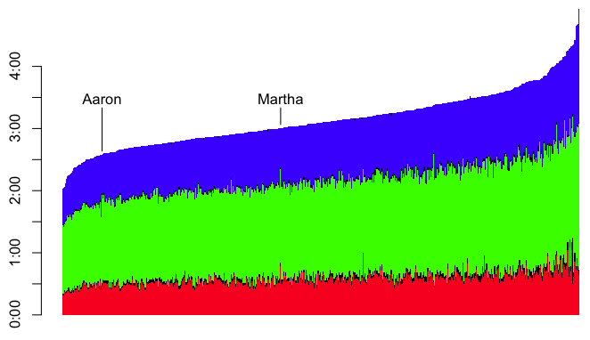
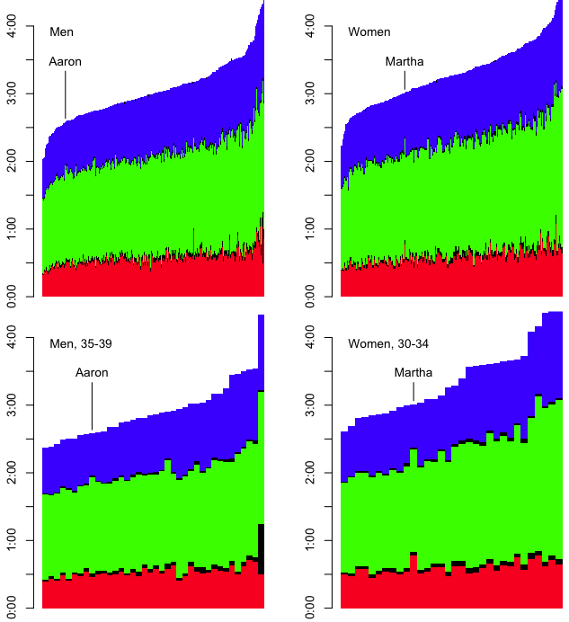
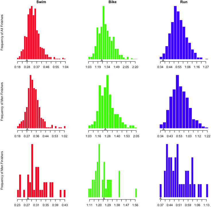
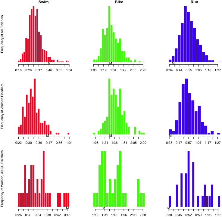
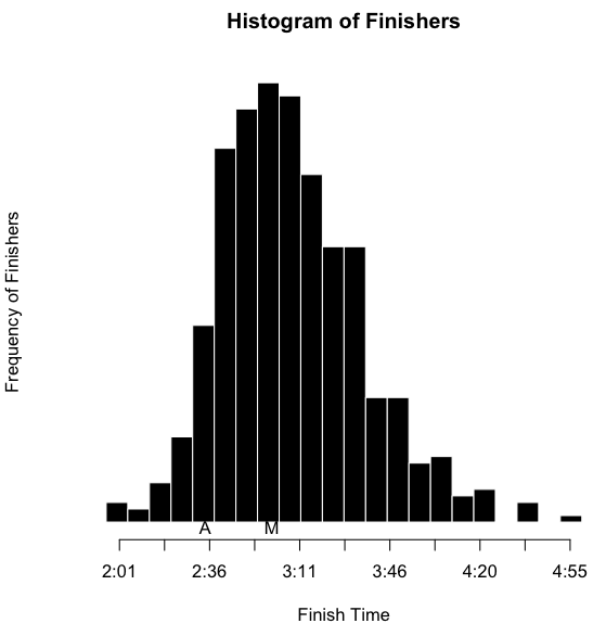
I’ve also inserted an ‘A’ below the results to notate where I finished, and an ‘M’ to notate where Martha finished. However, as I’ve indicated, part of the obsessing over the splits involves slicing the data as many ways as possible. I wanted to see this sort of histogram for each of the sports overall, by sex, and by age group. That’s a nine-way breakdown, for both me and Martha. Fortunately, since the data is all in R, and since I have the code all ready, it’s fairly trivial to make the histograms. They need to be viewed a bit larger than the width of this column, so you can click on the images below to see more detail. Here’s mine:

Luray Histogram, AaronLooking at my results, it is clear that I’m a stronger swimmer than cyclist, but it’s really the run that saves my race. Here’s Martha’s:

Luray Histogram, Martha

Notice that in her age group, she had the slowest swim, and the fastest run. She clearly gets stronger as the race goes on.

But there is still (at least) one more way to look at the results. Not only do we want to know how we perform in each of the disciplines; we also want to know how we progress through the race. That is, how do our positions change from the swim to the bike to the run to the finish? I started off with a function similar to “getSplits” above. I called this totalSplits. For a given racer, this produced a vector of the cumulative time after six points in the race: swim, t1, bike, t2, run, penalties. I could use those vectors to build a matrix, which I could then use to build a graph of how race positions changed from the swim to the bike to the finish.

all.totals <- t(matrix(apply(results, 1, totalSplits), nrow=6))
# Exclude results that are incomplete
all.totals <- all.totals[which(all.totals[,6] != 0),]
cnt <- length(all.totals[,1])

# Map the swim, bike, and finish times onto a range of 0 to 1, with
# 1 being the fastest, and 0 being the slowest.
doScale <- function(points) {
  1 - ((points - min(points)) / (max(points) - min(points)))
}
scaled.swim <- doScale(all.totals[,1])
scaled.bike <- doScale(all.totals[,3])
scaled.finish <- doScale(all.totals[,6])

# Plot points for swim, bike and finish places
plot(c(rep(1, cnt), rep(2, cnt), rep(3, cnt)),
     c(scaled.swim, scaled.bike, scaled.finish),
     pch='.', axes=FALSE, xlab='', ylab='',
     col=c(rep('red', cnt), rep('green', cnt), rep('blue', cnt)))

# Add the lines that correspond to individual racers
for (i in 1:cnt) {
  lines(c(1,2,3),
        c(scaled.swim[i], scaled.bike[i], scaled.finish[i]),
        col='#00000022')
}

# Add some axes
axis(1, at=c(1, 2, 3), labels=c('Swim', 'Bike', 'Finish'))
axis(2, at=c(0, 1), labels=c('Last', 'First'))

From that, I get something that looks like this:

Luray Results, Places

It looks like a crumpled piece of paper, so perhaps it needs some explanation. At the left is the placing for racers after the swim from the fastest swimmer at the top, to the slowest at the bottom. In the middle is the placing after the bike, and on the left is the placing at the finish. The first thing I notice is that there seems to be little correlation between placing after the swim and after the bike. The left side of the graph looks like a jumbled mess. The other thing I notice is that the top racers — note that prize money brought some pros to this race — are fantastic all-around. To pick out my results and Martha’s results, I highlighted them in aqua and yellow, respectively.

And for the sake of completeness, we need to break that down by sex and age group.

Luray Placing by Sex and AG

So yes, I suppose the moral of the story is that no one can obsess over results like a triathlete can obsess over results.

And in case anyone wants to play with the results, click the link to get the CSV of the results for the 2014 Luray International Distance Triathlon.

running

Hellgate Overview

[The following is an overview of the Hellgate 100k course. I originally wrote it in 2006, and I’ve amended it several times through the years. I’ve finished the race 11 times, so I don’t have much more to say about it, but I’ve decided to move the overview to this blog for the sake of content consolidation. D’I miss anything, or get it wrong? Feel free to append, extend, expand, propound, or offer your own observations in the comments.]

Hellgate 100k

Alrighty, folks. I was recently looking at a map of the Hellgate course to refresh my memory about how it goes. Then I realized that that was a terrible idea. I mean, after doing this race five times, the one thing you definitely don’t want to do is remember anything about it. But by the time I remembered that, it was too late. Yet the same desire that would make me say, “EWWW, taste this!” after drinking sour milk makes me want to share the memories. So here’s a handy little overview of Hellgate. (I should also note that Keith Knipling put together a far more high-tech overview of the 2007 race. Me, I use a highlighter and a map that I spread on my floor. Keith, he’s got heartrate data, GPS details and elevation profiles. How can I compete with that? I CAN’T, I TELL YOU! *sigh* So I just have to rely on my razor-sharp wit and boyish good looks to keep you interested in what I have to say.)

I’ll give you the full map immediately below. After that, I’ve broken it down, aid station to aid station. I’ll give you Horton’s description of each section, followed by the effluvia of my ruminations. In the map below, the race starts in the upper right, and follows the yellow highlighter generally toward the lower left. The start, finish and aid stations are marked with little red stars. The map I used for this little presentation is,

National Geographic Topographic Map #789
Lexington, Blue Ridge Mts
George Washington and Jefferson National Forests
Virginia, USA
Featuring: Glenwood / Pedlar Ranger District
ISBN: 1-56695-118-6
http://shop.nationalgeographic.com/product/615/803/246.html

I originally put together this overview before the 2006 race. During subsequent years, I realized that there were some sections that I needed to update because I had remembered some details incorrectly. But most of all, I realized that this sort of overview could be only marginally useful. Hellgate, more than any other race I’ve done, has a character that changes drastically from year to year. I’m not just saying that some years it’s chillier than other years. I’m saying that from year to year, this is a completely different race. One year, a certain section of the course might be particularly difficult, and the next year, that same section might be… less notable.

So far, we’ve had,

  • 2003 – The first year of the race, no one knew what to expect. The weather was cold, and there was a light fall of snow on the ground. The moon was full, and the sky was clear. With no leave on the trees, no clouds in the sky, and white snow on the ground, the moon lit up the trails like daylight. I turned on my flashlight for the more technical downhills, but I ran most of the way by the light of the moon. And the end of that first year, everyone knew we had been part of something special. And we were all amazed at just how difficult the race was.
  • 2004 – The “warm year” was different, in that there was no moon. I was quite comfortable in shorts. When I finished, I wondered how I could have forgotten just how difficult the race was.
  • 2005 – The “ice year” was just ridiculous. Several inches of snow fell early in the week. On friday, the temperature rose to the 60s, then fell at night to the 20s. Every road section was covered with glare ice, and every trail section had fluffy snow under a half-inch thick crust of ice. Staying upright was the name of the game. Just walking across the parking lot at Camp Bethel, from your car to race registration, was a harrowing experience. When I finished, I wondered how I could have forgotten just how difficult the race was.
  • 2006 – The “cold year” (or “the year of the leaves”) was when we learned that eyeballs can, in fact, freeze. With temperatures around 12°F at Headforemost mountain, and strong head winds, things got ugly. Four people ended up with severely impaired vision when their corneas froze later in the race. (After thawing out, everyone’s vision returned to normal.) Further, due to a lack of recent rain, leaves piled up as high as a foot and a half deep on many parts of the course. With uneven trail and loose rocks underneath, the leaves made footing extremely difficult. When I finished, I wondered how I could have forgotten just how difficult the race was.
  • 2007 – The “nice” year was probably as good as it gets. Most years, the 10 or 15 minutes before the race start, as we stand around in our Lycra® and our Polartec®, can be painfully cold. This year was rather nice. I was in shorts, and not particularly uncomfortable (which meant the temperature was in the upper 30s). There had been very little rain leading up to the race, so even the early creek crossing was a non-issue. There was a little bit of ice on some of the roads at higher elevations early in the race, and there were some deep leaves covering trails later in the course, but neither was as bad as previous years. We finally had a year when we could judge whether the race was difficult because of the weather of previous years, or because the course was just that hard. I’ll let you guess what the conclusion was. But I’ll give you a hint: about two seconds after I crossed the finish line, I was flat on the ground. Oh yeah, and when I finished, I wondered how I could have fotgotten just how difficult the race was. (Though I should mention that this year was a very special race for me. The full story is here.)

Are you picking up on the theme here?

Hellgate 100K Course

read more »

electronics

An Arduino-Based Computer For The Jeep

In my early 20s, I made what, at that point, was the biggest purchase of my life: my little, green Volkswagen. In both a literal and figurative way, it carried me through some formative years. After 11 years, when repair bills were starting to exceed the value of the car, it finally became time to retire The Green Machine. (It wasn’t an easy decision, but I got a very large estimate to weld out a bad catalytic converter, and weld in a new one that would be necessary to get the car to pass its emissions inspection.) In its place, I wanted something that would handle snowy mountains a bit better — that meant four-wheel drive — and something that I could pay for in cash without totally draining the kitty. I ended up with an 11 year old Jeep Wrangler.

The Jeep has several drawbacks over the Volkswagen. It’s loud. It’s a rough ride. Despite seeming to be quite a bit larger, it doesn’t have much carry capacity at all — packing the car for any long trip becomes an exercise in applied geometry and spacial relations. However, it does have one big advantage: it is user serviceable. It’s a great car for modification and personalization. All cars should be so modular. When a side mirror recently broke, my only problem was deciding what kind of mirror I wanted to replace it with. I browsed through the options on Quadratec, picked a set, they arrived two days later, and it took me 20 minutes to replace both mirrors. When I decided that the stock headlights were too dim, I bought new enclosures for a different bulb type, and swapped the old for the new. Busted radiator? Got a new one at the local auto parts store, and swapped it out. Want seat heaters? Add a fuse block, and wire them to switches on the dashboard. (I’m sure I’ll post more about that one later.)

Since I’ve been driving the Jeep, one feature of the VW I have longed for is the little computer that would tell me the temperature outside, how long I have been driving, and my average speed. Maybe I care too much for stats, but I liked to know, eg, This trip was 19 miles, it took 26 minutes, and it is 68° F outside. The Jeep doesn’t even have a clock on the dashboard. No, to be able to see the time, I need to leave the radio (also an aftermarket replacement) on the clock display.

I finally took up the challenge to put together something that would give me the information I so yearned for. I decided to use an Arduino as the microcontroller for the project. I went to my other favorite site, Adafruit, and ordered most of the parts I’d need, such as a digital temperature sensor, a GPS shield, and a touchscreen display. When the parts arrived, it was time to get soldering.

Parts to solder

I had to solder the header pins to the GPS shield, and a set of wires to both the GPS shield and the touchscreen in order to connect them to each other. I didn’t want to connect them directly. The plan was to set it up so the microcontroller/GPS unit would be hidden under the dashboard. The display would be affixed to the top of the dashboard. The temperature sensor would be mounted to the front of a front wheel well, and wires would be run back through the engine compartment, and through a small hole I had drilled in the firewall. But before I could do all of that, I wanted to make sure the basic unit worked. Once I figured out how to interface with the temperature sensor, the touchscreen, and the GPS, it wasn’t particularly challenging to write code to pull data from the sensors, and spit the information to the display. I connected the display to the microcontroller/GPS unit through a breadboard, and plugged a 9V battery into it. It was a self-contained unit that I could plop on top of the dashboard.

Computer on dash

I’m holding the display, which is connected (through the breadboard) to the GPS shield which is plugged in to the Arduino, which is powered by a 9V battery. The display shows the time of day at the top. On the left is the outside temperature (“??? F” since it is not currently connected to the temp sensor), current speed, and altitude above sea level. On the right is current trip information: time, distance, and average speed (“0.0 MPH” because of a bug in my code at that time). At the bottom is the latitude and longitude, and a green dot, indicating that the GPS has a fix.

Once I was generally satisfied with how the device was working, I needed to replace the breadboard with a more convenient connection. I needed to connect nine wires, so I started digging around for a standard RS232 serial cable with a DB9 connector on both ends. Fortunately, I keep around all sorts of old cable that will probably never be useful again. After digging around the box, I found a cable with DB9 connectors. I tested all the pins to make sure that I had a serial cable — where there is a one-to-one connection between pins on each end — and not a null modem cable — where a pin on one end might be connected to multiple pins on the other end. I was in luck; the cable would work. I picked up some solderable DB9 connectors from Radio Shack, and put one end on the display, and the other end on the microcontroller.

For the temperature sensor, I needed to be able to plug in three wires. I like the simplicity of a standard 1/8″ stereo jack, so I soldered a female end to the wires on the microcontroller, and a male end to the wires from the temperature sensor. So that’s an easy-peasy-parcheesi connection! The only trouble I had with the temperature sensor was joining the wires that ran through the engine compartment. The sensor itself is wrapped in a waterproof casing, and is connected to a 1 meter wire. But that wasn’t long enough to make it to the cabin. Joining longer wires to complete the run was not a problem, but securing them from the elements was a concern. So I picked up some dual-layer heat-shrink. Standard heat-shrink will shrink tightly around a join, but it’s still possible that moisture could get in. Dual-layer heat-shrink has an internal layer of adhesive that melts at a temperature lower than the application temperature. The adhesive fills in the gaps, and creates a waterproof layer — it’s preferable to standard heat-shrink for outdoor applications. So I made the joins, heat-shrunk each of the three individual wires, and tested it. Everything worked fine. I added one more layer of heat-shrink around all three wires, and tested again. The sensor no longer worked. I suspect that I over-heated the wires. Rather than using a proper heat gun, I was just waving a lighter under the heat-shrink. I think I was over zealous in my attempts at shrinkage, and I somehow ruined the connections or wires with too much heat. I had to cut out the connection, pull the remaining wires closer together, and start over. Eventually, I got it right.

Temperature Sensor

Clockwise from top left: 1) Under the front, drive-side wheel well. The white wire is connected to the temperature sensor. The sensor itself is on the left, wrapped in black Gorilla Tape, to add extra insulation against the elements. 2) Under the hood, the white temperature sensor wire comes from the bottom left up to the point where it is joined (with a length of black heat-shrink) to red, black, and green wires that run to the back of the engine compartment and through the firewall. 3) The wires from the temperature sensor terminate at a 1/8″ stereo plug.

For the GPS, I needed an external antenna, as the GPS chip would eventually be placed under the dash, where it would have a hard time finding a signal. I got an external, active antenna that I could place someplace where it would have good line-of-sight to the satellites. I found that the best location was on top of the dashboard. That made it easy to run the wire behind the dashboard, down to where the microcontroller would eventually be living. The antenna wire ends in an SMA connection (which is a small coax-type connection), so I us an SMA to uFL adapter to connect it to the uFL connector on the GPS shield.

The antenna is mounted on the dashboard. The wire runs behind the dashboard, and terminates in an SMA connector, which is connected to a uFL adapter.

The antenna is mounted on the dashboard. The wire runs behind the dashboard, and terminates in an SMA connector, which is connected to a uFL adapter.

The final piece of the puzzle was power. Fortunately, for other purposes, I had previously installed an extra fuse box in the Jeep, and I had a few spare switched (ie, on when the car is on; off when the car is off) leads in the cabin. I connected one to a 2.1mm power connector, and that was all I needed to do to power the microcontroller. However, when I took the whole contraption for a ride, I noticed that the Arduino ran very hot. The car provides a fairly dirty 12-14 volts, with possible spikes that could get to 18 or 20 volts. Based on the Arduino specs, the on-board voltage regulator should be able to handle that. But aside from my own observation that the device became worryingly hot, research seemed to indicate that it was only a matter of time before I fried the device. So I decided that I’d try to feed it a clean 7 or 9 volts. (It needed to be at least 7V because the GPS shield required 5V, and the on-board regulator would cause a drop of at least 1.5V from whatever I supplied.) I considered cheaping out, and just adding a standard, 7807 or 7809 voltage regulator. But in case I end up packing everything together in a tight space, I didn’t want to have the heat dissipation issues of a voltage regulator, so I went with a much-more-expensive buck converter. Whereas a voltage regulator reduces voltage by dissipating excess energy as heat, a buck converter is a highly efficient electronic device that will step down voltage with minimal waste. I hunted down a Traco TSR 1-2490 and installed it inline with the power connector.

A Traco TSR 1-2490 buck convert is connected inline with the power connector to supply a clean 9 volts.

A Traco TSR 1-2490 buck convert is connected inline with the power connector to supply a clean 9 volts.

Since I haven’t finalized the installation, the cockpit of the car is a mess of wires that I can connect to the microcontroller when I put it into the car.

mess_of_wires

And the controller itself is sort of a mess (but somewhat less delicate that you’d think — yay for solid solder joints!).

The Whole Kielbasa

But hey, it works! So the next step is to make some custom enclosures, and tidy everything up. I have some ideas, but I might not get around to it for a few months.

Display

bike

A New Old Bike

In the late 90s, my parents gave me a Specialized Crossroads A1 Expert hybrid bike. At the time, it was the nicest bike I had ever owned — aluminum frame and 7-speed with a triple (or “21-speed” depending on your preferred nomenclature). I would tool around on the bike paths for a few miles at a time, and eventually, I trained for my first triathlon on that bike (though I did the race on a borrowed road bike).

In the years since then, I’ve had an array of bikes — triathlon, road, fixie, mountain bike — each serving a different purpose. Several years ago, my father asked if I was using the Crossroads, and if I wasn’t, he was interested in taking it so he could run short errands on it. He used it for a while, but for the past few years, the bike has been sitting in my parents’ garage, unused and unloved.

The last triathlon I did was an iron-distance race in 2008. In 2009 and 2010, I was focused on running, and since then, I had been so exhausted with Lyme disease that I could never muster the energy to do much swimming or biking. But a few changes have gotten me back on the bike:

  1. Since addressing the whole Lyme thing, I’m returning to my old energy levels.
  2. Spending a week crewing for my friend, Kiwi Chris, as she completed a quintuple iron-distance triathlon (12 mile swim, 560 mile bike, 131 mile run) made me nostalgic for all the good times and adventures she and I had on the bike over the years, and I realize how much I missed riding.
  3. I continue to have severe bursitis in both of my heels. I’m fairly certain that the inflammation was originally due to the Lyme, but at this point, it is somewhat chronic. My heels are better than they were a year ago, but it is entirely possible that it could be years — if ever — before I can run entirely pain-free. So my weekly running mileage is dictated by what my heels can handle. But biking doesn’t seem to cause pain or problems.
  4. Martha has been struggling with a few running-related injuries that have similarly limited her weekly mileage. So I’ve been introducing her to the joys (though she might use a different word) of swimming and biking.

To get in a few miles on the bike, I found a reasonable route to the office, and I started bike commuting occasionally. Living in Washington, DC, and commuting on a route that takes me over bumpy, pot-holed roads, craggy sidewalks, and a little bit of dirt, I’d use my mountain bike for the ride. It was a bit of overkill, but I decided that it would be better for my wee, little bum than trying to ride my road bike. Since I wasn’t doing much road riding, I left the road bike in storage, and I’d keep the mountain bike in the bike storage room of the co-op  where I live.

One day, when I went to get my mountain bike, I found an empty space in the bike storage room when my bike had been. The door leading outside from the bike storage room had been having trouble with the lock, so I assume that someone had come in from outside and picked the nicest bike in the room to steal. At the same time, Martha was getting more interested in riding (or at least, becoming a more willing participant). So I had pulled my road bike out of storage, and taken indefinite loan of a friend’s old bike for Martha to ride. Operation Ride More Bikes was in full swing, but we had hit several hitches:

  1. I was lacking a bike suitable for commuting to work.
  2. Aside from my non-existent commuter bike, we had two bike that could not be left in the bike room (since the bike room was clearly not secure), yet we live in an apartment that is barely big enough for two adults and a cat.

Before I could address point #1, I had to do something about point #2. Fortunately, we have high ceilings and solid walls. My first attempts to drill into the studs failed. But a new carbide drill bit made quick work of it.


Bikes on a wall

A nuisance becomes an objet d’art! The cat approves.

Once I had gotten the road bikes out of the way, I could focus on my commuter. The old Crossroads was available.

Bike before

The frame was perfectly good, but the 7-speed drivetrain was due for an overhaul. Further, I don’t like riding in tight spaces with straight handlebars. I started spec’ing out parts to turn it into a cyclocross-style bike. I didn’t want to pour thousands of dollars into it, but I wanted to build a bike that could take a beating and would last. I considered going with Campy or SRAM, but I’ve always used Shimano, so I stuck with what I know. I like the 105 line as a good compromise between price and quality. So I ordered a bunch of parts — a new bottom bracket, cranks and chainrings, a cog set, deraillures, levers — and started to strip down the bike.

Stripped bike

Getting out the bottom bracket was the hardest part. It was seized with 16 years of dirt and grime. Fortunately, some WD-40 and a 24″ breaker bar did the trick.

My strategy was to replace only as much as necessary to convert the bike to a Shimano 10-speed drive train (with a double) and drop handle bars. I had to hunt around a bit for an inexpensive rear wheel that would fit the 135mm dropouts, but once I had that, I was ready to go. The build-up was pretty easy.

My new bike

As much as it sucked for my mountain bike to be stolen, I’m really, really happy with my new old bike. It brings together the best qualities of my mountain bike (softer ride) and my road bike (faster ride) when cruising around the city.

There are a few to-do items remaining for the bike, but none of them is stopping me from riding the steed.

  1. New pedals: I currently have platform pedals with single-sided SPD attachments. I’d prefer double-sided SPD pedals with no platform.
  2. New brakes: I considered picking up some new brakes, but I decided that it wasn’t absolutely necessary. The current brakes are old, but still functional. If the bike works out, next summer, I’ll upgrade. For now, I just put in new pads.
  3. New stem: This was my biggest miscalculation. I didn’t realize that modern drop bars have a different diameter at the center than old drop bars. None of the old quill stems I had laying around would work with the new bars. So I had to order a quill stem adapter, and a new stem. The stem I got is 100mm, but it turns out that that’s too long. To avoid being overly stretched out, I have to jam the seat way forward. It’s not an ideal fit, but it works for now. Again, if the bike works out in the long term, I’ll pick up a 50mm stem and fix the fit.
  4. New headset and fork: The headset is in terrible condition. It’s still smooth, but externally, there’s quite a bit of rust. If I had a headset press handy, I’d probably take care of this sooner rather than later. However, I’ll either need to borrow the tools from someone, but build my own DIY headset press. (I do few enough headsets that I don’t want to pay an extra $100-$150 just for the tools.) Whenever I do the headset, I’d like to convert to threadless, and replace the fork as well.
  5. New seat post: This is purely aesthetic, but I think I’d be happier with a clean, matte black seat post. Maybe I’ll just wrap the current post with electrical tape and call it a day.
  6. New deraillure hanger: The deraillure hanger is slightly bent, which means that if I were to shift into my biggest cog (easiest gear), the spokes on the rear wheel would rip off the chain tensioner. For now, I have the limiters set so I don’t accidentally cause that to happen.

I wanted to take some pictures of the bike all shiney and new, but actually riding it took precedence. So these pictures are after a few rides (and one commute to work). Please excuse the shmutz.

Drivetrain

Levers

Breaks

Stem

Saddle