After spending a few days in south-western Montana for the Fools Gold 50 Miler (which was rerouted into a 50k mid-race when race management found that Friday night’s snowfall (in August — yes, I know!) made the high ridges impassable, or at least unsafe), Martha and I headed to Yellowstone for a few days of critter tracking. I tend to be a light packer, so I don’t usually travel with the “good” camera. But Yellowstone seemed worthy of an exception. By the time I had crammed my luggage with the 7D body, the 70-200mm f/2.4 lens, the 2x lens extender, and a wide lens, camera gear probably constituted a third of the mass of my bag.
The wide lens ended up being almost entirely unused. Although Yellowstone has some amazing landscapes, our trip motto became, “BOO geology, YAY biology!” We were much more interested in hiking on lightly used trails in search of some small sparrow we hadn’t yet seen, rather than join the hoards of tourists gathering to gaze at geysers. Eventually, despite Martha’s initial desire to see bears, we grew weary of our fellow park visitors who were only interested in large game — bears, wolves, and bison. In a pond by the side of a road, Martha and I were watching a white pelican scoop up fish, surrounded by buffleheads, when a pair of sandhill cranes came in for a landing on the opposite shore. We marveled at the scene, when a car pulled up.
“What is it?” they asked. We explained what we were observing. “Oh,” they responded in disappointment, “we want to see wolves.” Then they drove off.
We spent some time driving, looking for roadside attraction, as is the practice at Yellowstone. But we spent much more time hiking on trails where we saw few people. We walked slowly, trying to spot every bird or small mammal that rustled a leaf, or made a barely audible peep on the trail. And like hunters “bagging” game, we were getting photos as prizes of the critters we encountered.
The photo inventory of our animal sightings not only had the benefit of providing a record of the trip. It also allowed after-the-fact consultation with our go-to bird expert, Martha’s brother, Fred. While Martha was able to identify about 80% of the birds we saw, the obscure, the western, and the juveniles (which often have entirely different coloration from the adults) occasionally eluded her. (I, on the other hand, have the a level of expertise that only allows me to call out, “BIRD!” upon seeing some vaguely bird-shaped creature.)
In whittling down the pictures to a set small enough that it might have interest for casual viewers, I briefly considered creating a gallery consisting of all pictures I took of animals looking directly at the camera. While I could have put together a fair sized gallery of those pictures, I decided that that would force me to exclude higher quality images for lower quality images in order to meet an arbitrarily imposed criterion. Instead, I picked a collection of favorites that provides a representative sampling of what we saw. (Pictures are clickable for larger versions.)
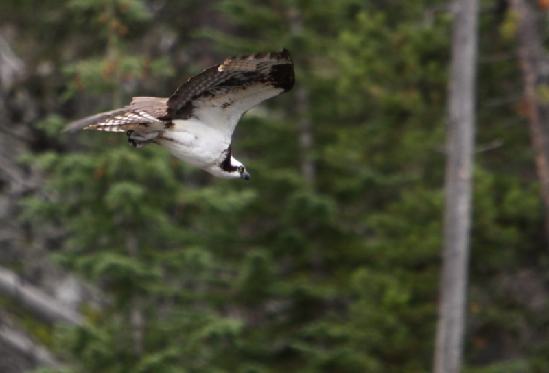
Osprey in Flight
Early on the first day, while driving down a narrow road by a stream, Martha asked me to stop. I pulled into the next pull-off (which are abundant in Yellowstone for exactly this reason). We walked back up the shoulder of the road to find a large osprey she had spotted in a tree. I got a couple shots of it in its perch before it started to fly. This was one of the first shots I took, as it swooped down in front of us. I spent a while trying to get a good Osprey In Flight photo on the second day when we happened upon several birds flying over a lake, not realizing I already had such a good one.
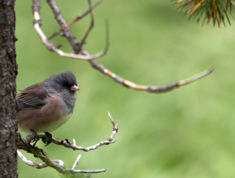
Junco
I’ve learned to recognize the juncos by the long, black and white tail feathers. That’s usually all I see as the flitter about in the shrubs. I had never seen one stay still for long enough for me to get a good look at it. They’re actually much more interesting — with the reddish, blueish, brownish coloration — than I had realized.

Red Squirrel
The red squirrel made the cut due to abundance rather than exoticness. These guys don’t like it much when you encroach on their territory. They’ll yell at you with a long, rattley-chirpy kind of sound. This guys seemed particularly peeved by our presence.
Juvenile Bald Eagle
The second day started much like the first day: with Martha excitedly asking me to pull to the side of the road. She had spotted a large bird in a tree, as we passed at relatively high speed. She said it might be another osprey, but we had all day, so it was worth a look. We found this bird, which is clearly not an osprey. She thought it might be a juvenile bald eagle, only because it was the right size, and we were in the right part of the park. When we reached a ranger station, we found a bird book, and confirmed that it was a juvenile (2nd year) bald eagle. (We later double-confirmed with Fred.)
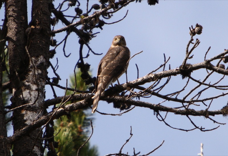
Sharp-Shinned Hawk
I noticed this one early in our hike on the second day. While tracking it as it flew from tree to tree, some other hikers came wandering down the trail, discussing the turmoil in Ukraine and Russia. One of them asked, “Anything interesting up there?” I pointed out the hawk. “Okay,” he replied in a tone that suggested he was annoyed that his conversation had been interrupted for something so pedestrian (metaphorically speaking, that is).
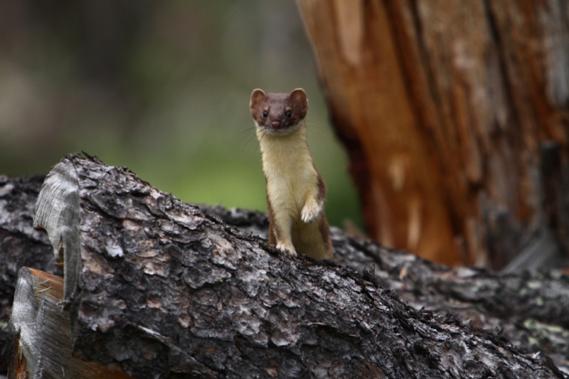
Long Tailed Weasel
After taking a break to eat some peanut butter sandwiches we had packed, Martha started hiking again; I was a moment behind. When I reached her, she was frozen with excitement. “AARON! I JUST SAW A WEASEL!” There was a moment when we both were beginning to lament that I wasn’t at the ready with the camera before the weasel disappeared. But then it popped its head out of the brush to inspect the human interlopers disturbing its forest. I got a picture before it disappeared again. Then it appeared again on the other side of a log, and disappeared yet again. It seemed to have a difficult time deciding whether to be fascinated by or terrified of us. In any case, I got several pictures of it inspecting us from various vantage points. To this day, Martha will still, apropos of nothing, blurt out, “That weasel was sooooooooo great!”
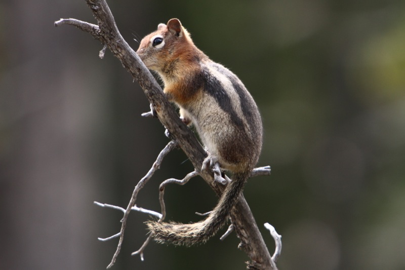
Golden Mantled Ground Squirrel
Sticking with the small mammals for a moment, this one was good enough to pose in nice light. Unfortunately, he (she?) skeetered away before I was able to move into a position where his (her?) little snout wasn’t obscured.

Trumpeter Swan
They mate for life, so that’s kind of interesting. This is one of the second pair of swans we came across.

Golden Eagle
Most of the time when I call out, “BIRD!” Martha informs me that it’s a crow or a vulture. Yellowstone has an abundance of ravens, so during this trip, I became an expert raven spotter too. Large, black birds seems to be my specialty. I noticed this bird flying overhead during the hike, and I attempted to take a picture because 1) it seemed like quite a large bird, and 2) I was honing my birds-in-flight photography skills. Neither of us got a good enough look at it against the bright sky to recognize it, and we couldn’t make it out by reviewing it on the camera’s viewfinder (particularly difficult on a bright day). A moment later, we smelled a dead animal, and noticed some vultures overhead. We decided it must have been another one of my famous vulture spottings. So you can imagine my delight when, in later review, Fred declared it to be a golden eagle.
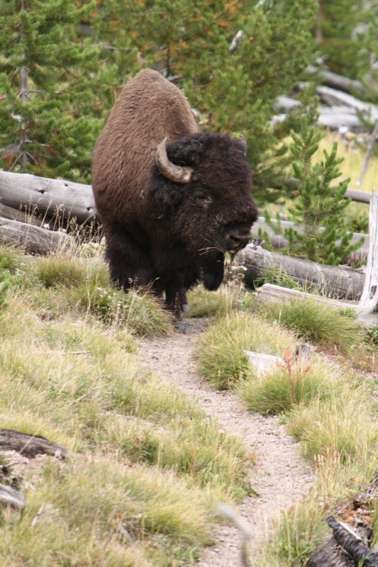
Bison
If you go to Yellowstone, there are two sights you can be sure you’ll see: geysers and bison. Just drive around a bit, and you’ll see each from the safety of your car. The thing about bison, you’ll hear over and over, is that you need to be careful around them. They seem like gentle giants who don’t mind all the people staring. However, if you get too close, they can be mean, angry, 1,200 lbs of beast. We were on a lightly used trail when we came around a corner to see this guy walking toward us along the trail. This was the second “sighting” of this sort in 30 minutes for us, so we wasted no time beating a path through the brush to give the bison a wide berth as we wondered whether our bear spray would work on a bison.
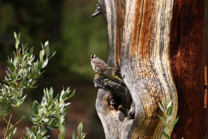
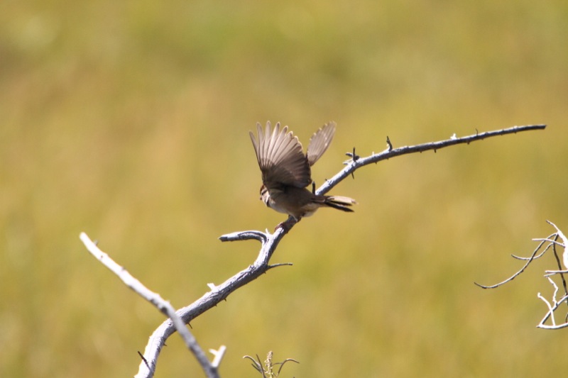
White Crowned Sparrow
Props to the bird for posing in such nice light!
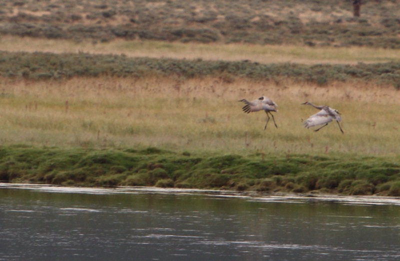
Sandhill Cranes
We saw several of these cranes flittering about. It’s not a fantastic shot, but I like their gangly legs as they are coming in for a landing.
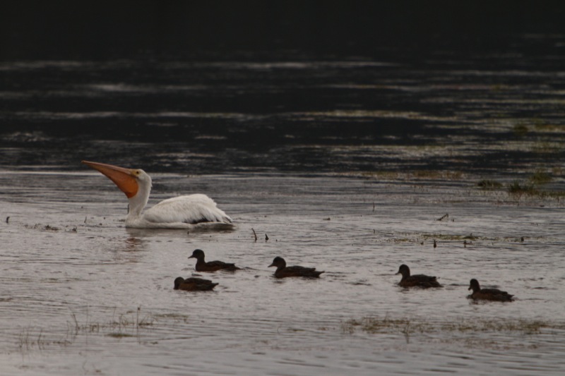
White Pelican
This bird was in a marsh by the side of the road. From a distance, we thought it might be another trumpeter swan, but they are normally found in pairs. We got closer to watch it scoop up dinner in its big beak (which, as they say, “holds more than its bellycan“).
Chipping Sparrow
By our third day, after seeing so many large and unusual birds, we start paying more attention to the small birds. We saw juvenile western tanangers, townsend’s warblers, western wood pewees, and a variety of other interesting, but easily overlooked, birds. (We also saw a steller’s jay that would have made a nice picture if it had been a bit more cooperative, and showed us more than its butt. We also saw a kestrel fly across a lake and land on a distant tree — too far to get a picture could show the bird as anything more than a few blurry pixels.) This chipping sparrow is probably one of the least interesting birds we saw, but I happened to click the shutter at exactly the right moment. This picture, therefore, is illustrative of two things: 1) a chipping sparrow, and 2) the fact that 10% of nature photography is technical skill while the remainder is split between patience and dumb luck.
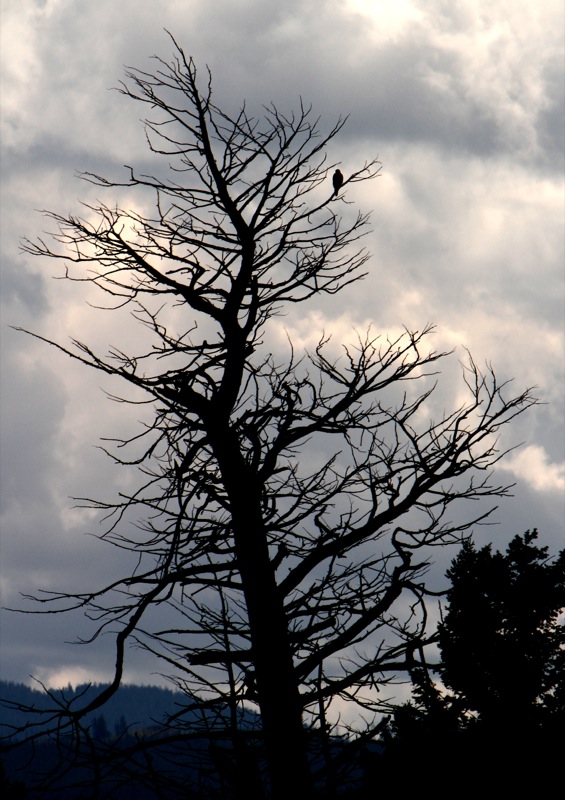
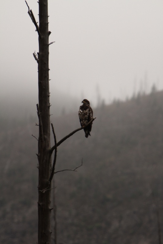
Bird In Tree
We have no idea what this one is, but I like the bird in the dead tree against the clouds. As I spent a few moments trying to get the exposure right, Martha kept telling me that it’s too far away, and that we wouldn’t be able to identify it. I told her, “I know, I KNOW! I’m just trying to do something here!”

Bald Eagle
And of course, there’s this guy. After sitting on the side of a road, watching several pronghorn antelopes gallop across a meadow, we were getting back into the car to move along when Martha spotted the eagle gliding across the sky, before it landed on a tree behind us. This was neither the first nor last bald eagle we saw during the trip. Still, I can never see an eagle without thinking of Gilbert & Sullivan.


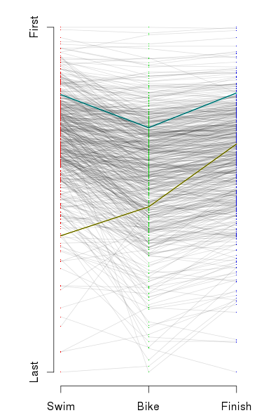
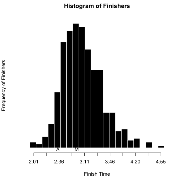 I’ve also inserted an ‘A’ below the results to notate where I finished, and an ‘M’ to notate where Martha finished. However, as I’ve indicated, part of the obsessing over the splits involves slicing the data as many ways as possible. I wanted to see this sort of histogram for each of the sports overall, by sex, and by age group. That’s a nine-way breakdown, for both me and Martha. Fortunately, since the data is all in R, and since I have the code all ready, it’s fairly trivial to make the histograms. They need to be viewed a bit larger than the width of this column, so you can click on the images below to see more detail. Here’s mine: